管部品模型集
Astropyモデルセットは、同じ(線形)モデルを多くの独立したデータセットに適合させることができます。このアルゴリズムは線形連立方程式を同時に求め,ループ演算を回避している.しかし,データを正しい形状に変換するのはやや困難である可能性がある.
節約された時間は努力する価値があるかもしれない。以下の例では、幅を変更すると データ立方体の高さを500に設定 500 2015年のMacBook Proでは、モデルセットを用いてモデルに適応するのに140ミリ秒を要した。同様のフィッティングを500*500モデル上で再帰的に行うことで1.5分と600倍以上遅れた。
以下の例では、3 Dデータ立方体を作成し、第1の次元はランプであり、例えば、赤外線検出器の非破壊読み取りによる。したがって、各画素には時間軸に沿った深さおよび流量が1つあり、これにより、カウントの総数が時間とともに増加する。一次元多項式と推定流量の時間を合算し,単位はカウント/秒(フィッティングの傾き)である.3行×4列の小画像のみを用い,深さは10個の非破壊読み取りである.
まず,必要なライブラリを導入する:
>>> import numpy as np
>>> np.random.seed(seed=12345)
>>> from astropy.modeling import models, fitting
>>> depth, width, height = 10, 3, 4  # Time is along the depth axis
>>> t = np.arange(depth, dtype=np.float64)*10.  # e.g. readouts every 10 seconds
各画素のカウント数は、フラックス*時間にいくつかのガウス雑音を加えた:
>>> fluxes = np.arange(1. * width * height).reshape(width, height)
>>> image = fluxes[np.newaxis, :, :] * t[:, np.newaxis, np.newaxis]
>>> image += np.random.normal(0., image*0.05, size=image.shape)  # Add noise
>>> image.shape
(10, 3, 4)
モデルを作りクランプします同じ線形パラメータ化モデルのN=幅*高さのインスタンスが必要です(モデルセットは現在線形モデルおよびチューブにのみ適用されています):
>>> N = width * height
>>> line = models.Polynomial1D(degree=1, n_models=N)
>>> fit = fitting.LinearLSQFitter()
>>> print(f"We created {len(line)} models")
We created 12 models
私たちはデータを正しい形に適合させる必要がある。3 Dデータ立方体にデータを提供するだけでは不可能である.この場合、時間軸は1次元であってもよい。フラックスを一定の形状を持つアレイに組織しなければならない width*height,depth つまり、最後の2つの軸を平らにし、位置を交換して、それらを第1の位置に置くように再構築しています:
>>> pixels = image.reshape((depth, width*height))
>>> y = pixels.T
>>> print("x axis is one dimensional: ",t.shape)
x axis is one dimensional:  (10,)
>>> print("y axis is two dimensional, N by len(x): ", y.shape)
y axis is two dimensional, N by len(x):  (12, 10)
モデルに合う。同時にN個のモデルに適しています
>>> new_model = fit(line, x=t, y=y)
>>> print(f"We fit {len(new_model)} models")
We fit 12 models
配列は、最適適合から計算された値で充填され、元の:
>>> best_fit = new_model(t, model_set_axis=False).T.reshape((depth, height, width))
>>> print("We reshaped the best fit to dimensions: ", best_fit.shape)
We reshaped the best fit to dimensions:  (10, 4, 3)
モデルを調べてみましょう:
>>> print(new_model)
Model: Polynomial1D
Inputs: ('x',)
Outputs: ('y',)
Model set size: 12
Degree: 1
Parameters:
             c0                 c1
    ------------------- ------------------
                    0.0                0.0
    -0.5206606340901005 1.0463998276552442
     0.6401930368329991 1.9818733492667582
     0.1134712985541639  3.049279878262541
    -3.3556420351251313  4.013810434122983
      6.782223372575449  4.755912707001437
      3.628220497058842  5.841397947835126
    -5.8828309622531565  7.016044775363114
    -11.676538736037775  8.072519832452022
      -6.17932185981594  9.103924115403503
    -4.7258541419613165 10.315295021908833
       4.95631951675311 10.911167956770575

>>> print("The new_model has a param_sets attribute with shape: ",new_model.param_sets.shape)
The new_model has a param_sets attribute with shape:  (2, 12)

>>> print(f"And values that are the best-fit parameters for each pixel:\n{new_model.param_sets}")
And values that are the best-fit parameters for each pixel:
[[  0.          -0.52066063   0.64019304   0.1134713   -3.35564204
    6.78222337   3.6282205   -5.88283096 -11.67653874  -6.17932186
   -4.72585414   4.95631952]
 [  0.           1.04639983   1.98187335   3.04927988   4.01381043
    4.75591271   5.84139795   7.01604478   8.07251983   9.10392412
   10.31529502  10.91116796]]
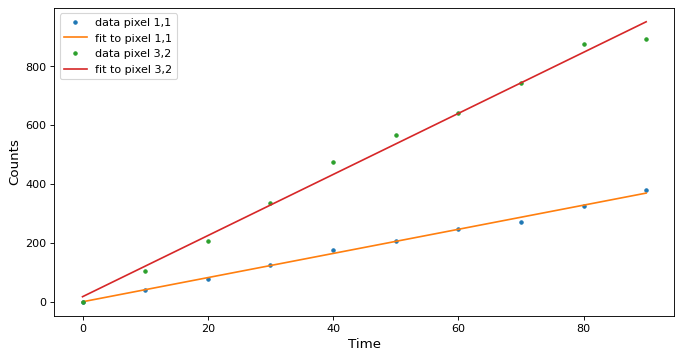
いくつかの画素に沿ってフィッティングを描きます
>>> def plotramp(t, image, best_fit, row, col):
...     plt.plot(t, image[:, row, col], '.', label=f'data pixel {row},{col}')
...     plt.plot(t, best_fit[:, row, col], '-', label=f'fit to pixel {row},{col}')
...     plt.xlabel('Time')
...     plt.ylabel('Counts')
...     plt.legend(loc='upper left')
>>> fig = plt.figure(figsize=(10, 5))
>>> plotramp(t, image, best_fit, 1, 1)
>>> plotramp(t, image, best_fit, 2, 1)
データは最適適合モデルとともに1枚の図に表示されている。
