制約を使ってフィッティングする
fitting 支持制約は、しかし、異なるチューブは、異なるタイプの制約を支持する。♪the supported_constraints 属性は、特定のクランプサポートの制約タイプを示します:
>>> from astropy.modeling import fitting
>>> fitting.LinearLSQFitter.supported_constraints
['fixed']
>>> fitting.LevMarLSQFitter.supported_constraints
['fixed', 'tied', 'bounds']
>>> fitting.SLSQPLSQFitter.supported_constraints
['bounds', 'eqcons', 'ineqcons', 'fixed', 'tied']
固定パラメータ制約
すべての部品はパラメータの固定(凍結)をサポートしています fixed パラメータをモデルに設定するか fixed 属性はパラメータに直接作用する.
線形フィッティングの場合、凍結多項式係数は、多項式係数を含まない多項式を結果に適合させる前に、データから対応する項を減算することを意味する。例えば修復は c0 多項式モデルでは,フィッティングデータに欠けている零級項からその定数を減算した多項式を用いる.固定係数と対応項は適合多項式に復元され,これは適合者から返された多項式である:
  >>> import numpy as np
  >>> np.random.seed(seed=12345)
  >>> from astropy.modeling import models, fitting
  >>> x = np.arange(1, 10, .1)
  >>> p1 = models.Polynomial1D(2, c0=[1, 1], c1=[2, 2], c2=[3, 3],
  ...                          n_models=2)
  >>> p1  # doctest: +FLOAT_CMP
  <Polynomial1D(2, c0=[1., 1.], c1=[2., 2.], c2=[3., 3.], n_models=2)>
  >>> y = p1(x, model_set_axis=False)
  >>> n = (np.random.randn(y.size)).reshape(y.shape)
  >>> p1.c0.fixed = True
  >>> pfit = fitting.LinearLSQFitter()
  >>> new_model = pfit(p1, x, y + n)  # doctest: +IGNORE_WARNINGS
  >>> print(new_model)  # doctest: +SKIP
  Model: Polynomial1D
  Inputs: ('x',)
  Outputs: ('y',)
  Model set size: 2
  Degree: 2
  Parameters:
       c0         c1                 c2
      --- ------------------ ------------------
      1.0  2.072116176718454   2.99115839177437
      1.0 1.9818866652726403 3.0024208951927585


The syntax to fix the same parameter ``c0`` using an argument to the model
instead of ``p1.c0.fixed = True`` would be::

  >>> p1 = models.Polynomial1D(2, c0=[1, 1], c1=[2, 2], c2=[3, 3],
  ...                          n_models=2, fixed={'c0': True})
有界制約
有界管通過 bounds モデルのパラメータや設定によって min そして max パラメータ上の属性。の境界です LevMarLSQFitter 常に完全に満たされている-パラメータの値が適合区間の外にあれば,境界上の値にリセットされる.♪the SLSQPLSQFitter 最適化アルゴリズムは内部で境界を処理する.
制約を制約する.
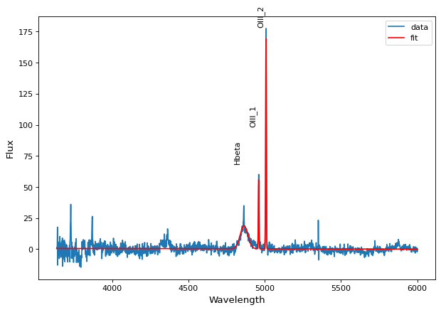
♪the tied 制約は通常対 Compound models それがそうです。この例では1つの名前から spec.txt OIII 1とOIII 2のスペクトル線のフラックスを連結しながら,ガウス関数をこれらのスペクトル線に同時にフィッティングした。
import numpy as np
from astropy.io import ascii
from astropy.utils.data import get_pkg_data_filename
from astropy.modeling import models, fitting
fname = get_pkg_data_filename('data/spec.txt', package='astropy.modeling.tests')
spec = ascii.read(fname)
wave = spec['lambda']
flux = spec['flux']

# Use the rest wavelengths of known lines as initial values for the fit.

Hbeta = 4862.721
OIII_1 = 4958.911
OIII_2 = 5008.239

# Create Gaussian1D models for each of the Hbeta and OIII lines.

h_beta = models.Gaussian1D(amplitude=34, mean=Hbeta, stddev=5)
o3_2 = models.Gaussian1D(amplitude=170, mean=OIII_2, stddev=5)
o3_1 = models.Gaussian1D(amplitude=57, mean=OIII_1, stddev=5)


# Tie the ratio of the intensity of the two OIII lines.

def tie_ampl(model):
    return model.amplitude_2 / 3.1

o3_1.amplitude.tied = tie_ampl


# Also tie the wavelength of the Hbeta line to the OIII wavelength.

def tie_wave(model):
    return model.mean_0 * OIII_1 / Hbeta

o3_1.mean.tied = tie_wave

# Create a Polynomial model to fit the continuum.

mean_flux = flux.mean()
cont = np.where(flux > mean_flux, mean_flux, flux)
linfitter = fitting.LinearLSQFitter()
poly_cont = linfitter(models.Polynomial1D(1), wave, cont)

# Create a compound model for the three lines and the continuum.

hbeta_combo = h_beta + o3_1 + o3_2 + poly_cont

# Fit all lines simultaneously.

fitter = fitting.LevMarLSQFitter()
fitted_model = fitter(hbeta_combo, wave, flux)
fitted_lines = fitted_model(wave)

from matplotlib import pyplot as plt
fig = plt.figure(figsize=(9, 6))
p = plt.plot(wave, flux, label="data")
p = plt.plot(wave, fitted_lines, 'r', label="fit")
p = plt.legend()
p = plt.xlabel("Wavelength")
p = plt.ylabel("Flux")
t = plt.text(4800, 70, 'Hbeta', rotation=90)
t = plt.text(4900, 100, 'OIII_1', rotation=90)
t = plt.text(4950, 180, 'OIII_2', rotation=90)
plt.show()