不確実性とその分布 (astropy.uncertainty )
注釈
astropy.uncertainty is relatively new (astropy v3.1), and thus it is possible there will be API changes in upcoming versions of astropy. If you have specific ideas for how it might be improved, please let us know on the astropy-dev mailing list Http://Feedback.asterpy.orgにアクセスしてください。
序言:序言
astropy 1つを提供します Distribution 対象は統計的分布を何らかの形で表しており,この形式は Quantity 対象や通常 numpy.ndarray それがそうです。このように使われています Distribution 追加的な計算を犠牲にして不確実性の伝播を提供する。例えば、モンテカルロ計算技術のためのサンプリング分布をより一般的に表すこともできる。
この機能の中心的な対象は Distribution それがそうです。現在,これらの分布はすべてモンテカルロサンプリングされている.これは,各分布がより多くのメモリを必要とする可能性があることを意味するが,分布関連構造を保持しながら分布に対して任意の複雑な操作を行うことを可能にする.いくつかの特定の行動の良好な分布(例えば、正規分布)は、最終的によりコンパクトかつ効率的な表現を達成することが可能な分析形態を有する。将来的にはこれらの技術は使用のための一貫した不確実性伝播機構を提供するかもしれません NDData それがそうです。しかし、これは現在施行されていない。したがって,不確実性の詳細な情報を格納する. NDData 相手は N次元データセット (astropy.nddata ) 一節です。
スタート
分布の基本用例を示すために,正規分布の不確実性伝播問題を考える.2つの測定値を追加すると仮定して、各測定値は正常な不確定度を持っています。いくつかの初期導入と設定から始めましょう
>>> import numpy as np
>>> from astropy import units as u
>>> from astropy import uncertainty as unc
>>> np.random.seed(12345)  # ensures reproducible example numbers
今私たちは2つの Distribution 対象は私たちの分布を表しています
>>> a = unc.normal(1*u.kpc, std=30*u.pc, n_samples=10000)
>>> b = unc.normal(2*u.kpc, std=40*u.pc, n_samples=10000)
正規分布については,中心は期待どおりに加算し,標準偏差は直交して加算すべきである.これらの結果を以下の命令で簡単に検査することができる(モンテカルロサンプリングの限界に達する) Distribution 算術と属性:
>>> c = a + b
>>> c
<QuantityDistribution [...] kpc with n_samples=10000>
>>> c.pdf_mean()
<Quantity 2.99970555 kpc>
>>> c.pdf_std().to(u.pc)
<Quantity 50.07120457 pc>
実は、これらは予想に近い。これは基本ガウスの場合には不要なようだが、誤差解析が成り立たなくなるより複雑な分布や算術演算では、 Distribution まだ通過できます:
>>> d = unc.uniform(center=3*u.kpc, width=800*u.pc, n_samples=10000)
>>> e = unc.Distribution(((np.random.beta(2,5, 10000)-(2/7))/2 + 3)*u.kpc)
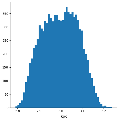
>>> f = (c * d * e) ** (1/3)
>>> f.pdf_mean()
<Quantity 2.99786227 kpc>
>>> f.pdf_std()
<Quantity 0.08330476 kpc>
>>> from matplotlib import pyplot as plt
>>> from astropy.visualization import quantity_support
>>> with quantity_support():
... plt.hist(f.distribution, bins=50)

Vbl.使用 astropy.uncertainty
配布を作成しております
分布を作成する最も直接的な方法は配列や Quantity サンプルを携帯して last サイズ::
>>> import numpy as np
>>> from astropy import units as u
>>> from astropy import uncertainty as unc
>>> np.random.seed(123456)  # ensures "random" numbers match examples below
>>> unc.Distribution(np.random.poisson(12, (1000)))
NdarrayDistribution([..., 12,...]) with n_samples=1000
>>> pq = np.random.poisson([1, 5, 30, 400], (1000, 4)).T * u.ct # note the transpose, required to get the sampling on the *last* axis
>>> distr = unc.Distribution(pq)
>>> distr
<QuantityDistribution [[...],
           [...],
           [...],
           [...]] ct with n_samples=1000>
この2つの発行版の違いに注意してください:最初の発行版は配列から構築されているのでありません Quantity 属性、例えば unit 一方,後者は確かにこれらの属性を持つ.これは他のオブジェクトとのインタラクションに反映されています NdarrayDistribution そんなことはありません。 Quantity 単位を含むオブジェクト。
一般的な発行版の場合、ヘルプ関数の存在は、それらを作成することをより容易にする。以下の例は、正規/ガウス分布を作成するいくつかの等価方法を示す。
>>> center = [1, 5, 30, 400]
>>> n_distr = unc.normal(center*u.kpc, std=[0.2, 1.5, 4, 1]*u.kpc, n_samples=1000)
>>> n_distr = unc.normal(center*u.kpc, var=[0.04, 2.25, 16, 1]*u.kpc**2, n_samples=1000)
>>> n_distr = unc.normal(center*u.kpc, ivar=[25, 0.44444444, 0.625, 1]*u.kpc**-2, n_samples=1000)
>>> n_distr.distribution.shape
(4, 1000)
>>> unc.normal(center*u.kpc, std=[0.2, 1.5, 4, 1]*u.kpc, n_samples=100).distribution.shape
(4, 100)
>>> unc.normal(center*u.kpc, std=[0.2, 1.5, 4, 1]*u.kpc, n_samples=20000).distribution.shape
(4, 20000)
また、ポアソンと制服 Distribution 作成関数存在:
>>> unc.poisson(center*u.count, n_samples=1000)
<QuantityDistribution [[...],
             [...],
             [...],
             [...]] ct with n_samples=1000>
>>> uwidth = [10, 20, 10, 55]*u.pc
>>> unc.uniform(center=center*u.kpc, width=uwidth, n_samples=1000)
<QuantityDistribution [[...],
             [...],
             [...],
             [...]] kpc with n_samples=1000>
>>> unc.uniform(lower=center*u.kpc - uwidth/2,  upper=center*u.kpc + uwidth/2, n_samples=1000)
<QuantityDistribution [[...],
             [...],
             [...],
             [...]] kpc with n_samples=1000>
ユーザは、同様のモードで自分の配信クラスを自由に作成することができる。
使用分布
この対象の現在の行動は非常に似ています Quantity あるいは…。 numpy.ndarray サンプリング次元以外のすべての次元については、サンプリング分布に機能する他の統計的動作が使用される:
>>> distr.shape
(4,)
>>> distr.size
4
>>> distr.unit
Unit("ct")
>>> distr.n_samples
1000
>>> distr.pdf_mean()
<Quantity [  0.998,   5.017,  30.085, 400.345] ct>
>>> distr.pdf_std()
<Quantity [ 0.97262326,  2.32222114,  5.47629208, 20.6328373 ] ct>
>>> distr.pdf_var()
<Quantity [  0.945996,   5.392711,  29.989775, 425.713975] ct2>
>>> distr.pdf_median()
<Quantity [   1.,   5.,  30., 400.] ct>
>>> distr.pdf_mad()  # Median absolute deviation
<Quantity [ 1.,  2.,  4., 14.] ct>
>>> distr.pdf_smad()  # Median absolute deviation, rescaled to match std for normal
<Quantity [ 1.48260222,  2.96520444,  5.93040887, 20.75643106] ct>
>>> distr.pdf_percentiles([10, 50, 90])
<Quantity [[  0. ,   2. ,  23. , 374. ],
           [  1. ,   5. ,  30. , 400. ],
           [  2. ,   8. ,  37.1, 427. ]] ct>
>>> distr.pdf_percentiles([.1, .5, .9]*u.dimensionless_unscaled)
<Quantity [[  0. ,   2. ,  23. , 374. ],
          [  1. ,   5. ,  30. , 400. ],
          [  2. ,   8. ,  37.1, 427. ]] ct>
必要であれば distribution 属性::
>>> distr.distribution
<Quantity [[...1...],
           [...5...],
           [...27...],
           [...405...]] ct>
>>> distr.distribution.shape
(4, 1000)
A Quantity distribution interacts naturally with non-Distribution
Quantity objects, assuming the Quantity is a Dirac delta distribution:
>>> distr_in_kpc = distr * u.kpc/u.count  # for the sake of round numbers in examples
>>> distrplus = distr_in_kpc + [2000,0,0,500]*u.pc
>>> distrplus.pdf_median()
<Quantity [   3. ,   5. ,  30. , 400.5] kpc>
>>> distrplus.pdf_var()
<Quantity [  0.945996,   5.392711,  29.989775, 425.713975] kpc2>
他の発行バージョンについても、予想通りに動作している(ただし、以下の共分散議論を参照)。
>>> another_distr = unc.Distribution((np.random.randn(1000,4)*[1000,.01 , 3000, 10] + [2000, 0, 0, 500]).T * u.pc)
>>> combined_distr = distr_in_kpc + another_distr
>>> combined_distr.pdf_median()
<Quantity [  3.01847755,   4.99999576,  29.60559788, 400.49176321] kpc>
>>> combined_distr.pdf_var()
<Quantity [  1.8427705 ,   5.39271147,  39.5343726 , 425.71324244] kpc2>
分布の共分散と離散サンプリング効果
分布の主な応用の1つは不確実性伝播であり,共分散を適切に扱う必要がある.これはモンテカルロサンプリングでは自然です Distribution クラスは,サンプリング誤差に適切に注意すればよい.
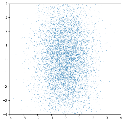
基本的な例から始めて、2つの非相関分布は、非相関共同プロファイルを生成するはずである。
>>> import numpy as np
>>> np.random.seed(12345) # produce repeatable plots
>>> from astropy import units as u
>>> from astropy import uncertainty as unc
>>> from matplotlib import pyplot as plt
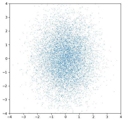
>>> n1 = unc.normal(center=0., std=1, n_samples=10000)
>>> n2 = unc.normal(center=0., std=2, n_samples=10000)
>>> plt.scatter(n1.distribution, n2.distribution, s=2, lw=0, alpha=.5)
>>> plt.xlim(-4, 4)
>>> plt.ylim(-4, 4)
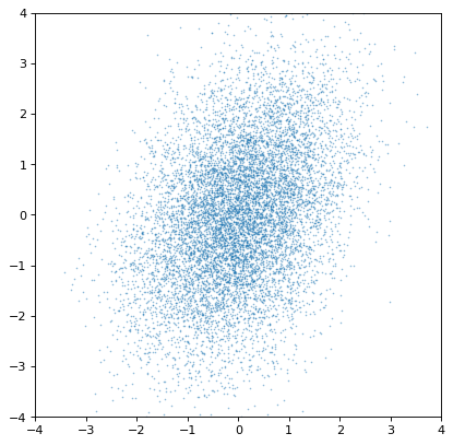
実際これらの分布は独立しています協力的なガウスを構築すればすぐに明らかになります
>>> ncov = np.random.multivariate_normal([0, 0], [[1, .5], [.5, 2]], size=10000)
>>> n1 = unc.Distribution(ncov[:, 0])
>>> n2 = unc.Distribution(ncov[:, 1])
>>> plt.scatter(n1.distribution, n2.distribution, s=2, lw=0, alpha=.5)
>>> plt.xlim(-4, 4)
>>> plt.ylim(-4, 4)
最も重要なのは、所望の適切な相関構造を適切な算術演算によって保持または生成することである。例えば、軸が独立でなければ、仮想的な恒星集合における鉄、水素、酸素豊富度のシミュレーションにおけるように、非相関正規分布の比率は共分散が得られる。
>>> fe_abund = unc.normal(center=-2, std=.25, n_samples=10000)
>>> o_abund = unc.normal(center=-6., std=.5, n_samples=10000)
>>> h_abund = unc.normal(center=-0.7, std=.1, n_samples=10000)
>>> feh = fe_abund - h_abund
>>> ofe = o_abund - fe_abund
>>> plt.scatter(ofe.distribution, feh.distribution, s=2, lw=0, alpha=.5)
>>> plt.xlabel('[Fe/H]')
>>> plt.ylabel('[O/Fe]')
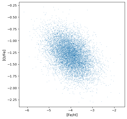
このことは,相関が変数に自然に生じることを示しているが,サンプリング過程が自然に存在する相関を回復することを明確に説明する必要はない。
しかしながら、1つの重要な警告は、サンプル軸がサンプル毎に完全に一致する場合にのみ、共分散を保持することができることである。そうでない場合、すべての共分散情報は(サイレント)失われる。
>>> n2_wrong = unc.Distribution(ncov[::-1, 1])  #reverse the sampling axis order
>>> plt.scatter(n1.distribution, n2_wrong.distribution, s=2, lw=0, alpha=.5)
>>> plt.xlim(-4, 4)
>>> plt.ylim(-4, 4)

さらに、サンプリング不足の分布は、より悪い推定または隠れ相関を与える可能性がある。以下の例は、上記の共変ガウス例と同様であるが、サンプル数は200倍減少している。
肉眼的には共分散構造はそれほど顕著ではなく,入力と出力共分散行列の間の有意差に反映されている。一般に,サンプル数が少ないほど計算効率が高いが,どの相関量においてもより大きな不確実性を招くサンプリング分布を用いた内在的なトレードオフである.これらは往々にして秩序がある \(\sqrt{{n_{{\rm samples}}}}\) どんな導出量でも、これは議論された分布の複雑さに依存する。
参照/API
占星術.不確定包
このサブパッケージは、動作モードと同様の発行版を作成するためのクラスおよび関数を含む Quantity あるいは配列オブジェクトであるが,不確実性が伝播する可能性がある.
機能
|
ガウス/正規分布を作成する。 |
|
ポアソン分布を作成する。 |
|
下界と上界から均一な分布を作る。 |
クラス
|
関連する不確実性分布を有するスカラ値または配列値。 |