画像の伸張と正規化¶

♪the astropy.visualization モジュールは、一般に視覚化目的のために、画像(およびより一般的な任意の配列)内の値を変換するためのフレームワークを提供する。2つの主なタイプの変換を提供しています

規範化されています [0:1] 下限と上限の範囲を使用して、 \(x\) 元の画像中の値を表す：

\[Y=\frac{x-v_{\rm min}{v_{\rm max}-v_{\rm min}}\]

伸びている 属性中の値の [0:1] 範囲から [0:1] 線形または非線形関数を使用する範囲：

\[Z=f(Y)\]

さらに、いくつかのクラスは、(例えば、パーセンタイル値を使用するような)特定のアルゴリズムに基づいてデータセットの下限および上限を決定するために提供される。

下限と上限を決定し，再正規化する過程について述べた。 Intervals and Normalization 部分的に拡張されています Stretching 一節です。

区間と正規化¶

ショートカット¶

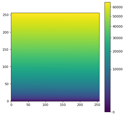
astropy 便利さを提供しました simple_norm() 高速相互作用分析に使用可能な関数：

import numpy as np
import matplotlib.pyplot as plt
from astropy.visualization import simple_norm

# Generate a test image
image = np.arange(65536).reshape((256, 256))

# Create an ImageNormalize object
norm = simple_norm(image, 'sqrt')

# Display the image
fig = plt.figure()
ax = fig.add_subplot(1, 1, 1)
im = ax.imshow(image, origin='lower', norm=norm)
fig.colorbar(im)

(png, svg, pdf)

この便利な関数は1つ結合しています Stretch オブジェクト、そして使用 Interval 相手。ご利用をお勧めします ImageNormalize この便利な関数ではなく、スクリプトプログラムで直接使用する。

詳細な方式¶

間隔を決定し、この間隔内の値を正規化するためのいくつかのクラスが提供される [0:1] 射程。最も簡単な例の1つは MinMaxInterval これは，配列中の最小値と最大値に基づいて値の制約を決定する.このようなインスタンス化にはパラメータがない：

>>> from astropy.visualization import MinMaxInterval
>>> interval = MinMaxInterval()

これらの制限は呼び出すことで get_limits() 方法、この方法は、値配列：

>>> interval.get_limits([1, 3, 4, 5, 6])
(1, 6)

♪the interval インスタンスは、値を実際に範囲に正規化するために関数のように呼び出すこともできる：

>>> interval([1, 3, 4, 5, 6])  
array([0. , 0.4, 0.6, 0.8, 1. ])

Other interval classes include ManualInterval, PercentileInterval, AsymmetricPercentileInterval, and ZScaleInterval. For these, values in the array can fall outside of the limits given by the interval. A clip argument is provided to control the behavior of the normalization when values fall outside the limits:

>>> from astropy.visualization import PercentileInterval
>>> interval = PercentileInterval(50.)
>>> interval.get_limits([1, 3, 4, 5, 6])
(3.0, 5.0)
>>> interval([1, 3, 4, 5, 6])  # default is clip=True  
array([0. , 0. , 0.5, 1. , 1. ])
>>> interval([1, 3, 4, 5, 6], clip=False)  
array([-1. ,  0. ,  0.5,  1. ,  1.5])

伸びている¶

値を小さくすることができることを除いて [0:1] 範囲内で、様々な関数を使用してこれらの値を“伸張”するために多くのクラスが提供される。これらの地図は [0:1] 変換されたものに広がっています [0:1] 射程。簡単な例として SqrtStretch クラス：：

>>> from astropy.visualization import SqrtStretch
>>> stretch = SqrtStretch()
>>> stretch([0., 0.25, 0.5, 0.75, 1.])  
array([0.        , 0.5       , 0.70710678, 0.8660254 , 1.        ])

間隔については [0:1] 範囲の処理方法は異なることができ、具体的には clip 論争する。デフォルトの場合、出力値は裁断されます [0:1] 範囲：：

>>> stretch([-1., 0., 0.5, 1., 1.5])  
array([0.       , 0.        , 0.70710678, 1.        , 1.        ])

しかし、この機能を無効にすることができます：

>>> stretch([-1., 0., 0.5, 1., 1.5], clip=False)  
array([       nan, 0.        , 0.70710678, 1.        , 1.22474487])

注釈

引張関数は似ていますが、常に厳密に同じではありません DS9 (同じ行動を持っているはずだが)。DS 9の伸びの方程式を見つけることができます here 拡張部分で与えられた方程式と比較することができます astropy.visualization API部分。私たちの伸展とDS 9の主な違いは私たちがそれらを調整したことです [0:1] 範囲は常に正確にマッピングされています [0:1] 射程。

組み合わせ変換¶

どの間隔やストレッチでもご利用いただけます + 演算子，この演算子は新たな変換を返す.間隔と引張を組み合わせた場合，引張対象は間隔対象の前に位置しなければならない。例えば、百分率値に基づいて正規化を適用し、平方根伸張を適用するには、以下の動作を行うことができる。

>>> transform = SqrtStretch() + PercentileInterval(90.)
>>> transform([1, 3, 4, 5, 6])  
array([0.        , 0.60302269, 0.76870611, 0.90453403, 1.        ])

前と同様に、組み合わせ変換も受け入れられます clip パラメータ(すなわち True デフォルトの場合)。

Matplotlib正規化¶

Matplotlibは伝達を通じて matplotlib.colors.Normalize オブジェクト、例えば imshow() それがそうです。♪the astropy.visualization module provides an ImageNormalize class that wraps the interval (see Intervals and Normalization )および伸張(参照 Stretching )オブジェクトはMatplotlib理解のオブジェクトに変換される.

入力します ImageNormalize クラスはデータおよびIntervalとStretchオブジェクトである：

import numpy as np
import matplotlib.pyplot as plt

from astropy.visualization import (MinMaxInterval, SqrtStretch,
                                   ImageNormalize)

# Generate a test image
image = np.arange(65536).reshape((256, 256))

# Create an ImageNormalize object
norm = ImageNormalize(image, interval=MinMaxInterval(),
                      stretch=SqrtStretch())

# or equivalently using positional arguments
# norm = ImageNormalize(image, MinMaxInterval(), SqrtStretch())

# Display the image
fig = plt.figure()
ax = fig.add_subplot(1, 1, 1)
im = ax.imshow(image, origin='lower', norm=norm)
fig.colorbar(im)

(png, svg, pdf)

以上のように、カラーバー目盛りは自動的に調整されます。

ご注意ください、誰も使うべきではありません ax.imshow(norm(image)) 色バー刻み度線は、実際の画像値ではなく、規格化された画像値(線形スケール)を表すからである。また、表示された画像 ax.imshow(norm(image)) 完全に同じではありません ax.imshow(image, norm=norm) もし画像が含まれていれば NaN あるいは…。 inf 価値観。正確な等価物は ax.imshow(norm(np.ma.masked_invalid(image)) それがそうです。

入力する画像 ImageNormalize 通常は表示されますので、便利な機能があります imshow_norm() この使用状況を簡略化するためには、以下の動作を実行してください。

import numpy as np
import matplotlib.pyplot as plt

from astropy.visualization import imshow_norm, MinMaxInterval, SqrtStretch

# Generate a test image
image = np.arange(65536).reshape((256, 256))

# Display the exact same thing as the above plot
fig = plt.figure()
ax = fig.add_subplot(1, 1, 1)
im, norm = imshow_norm(image, ax, origin='lower',
                       interval=MinMaxInterval(), stretch=SqrtStretch())
fig.colorbar(im)

(png, svg, pdf)

これは最も簡単な場合であるが、完全に異なる画像を使用して規格化を確立することもできる(例えば、完全に同じ規格化および伸張されたいくつかの画像を表示する場合)。

入力します ImageNormalize クラスはvminとvmax制限でもあります Intervals and Normalization クラスとStretchオブジェクト：

import numpy as np
import matplotlib.pyplot as plt

from astropy.visualization import (MinMaxInterval, SqrtStretch,
                                   ImageNormalize)

# Generate a test image
image = np.arange(65536).reshape((256, 256))

# Create interval object
interval = MinMaxInterval()
vmin, vmax = interval.get_limits(image)

# Create an ImageNormalize object using a SqrtStretch object
norm = ImageNormalize(vmin=vmin, vmax=vmax, stretch=SqrtStretch())

# Display the image
fig = plt.figure()
ax = fig.add_subplot(1, 1, 1)
im = ax.imshow(image, origin='lower', norm=norm)
fig.colorbar(im)

(png, svg, pdf)

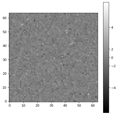
ストレッチとMatplotlibを組み合わせて規格化する¶

延伸は変換のように他の延伸と組み合わせることもできる。ここから生まれたのは CompositeStretch 規格化Matplotlib画像は他のどのような延伸のように使用することができる。例えば、複合延伸は、負の値を有する残差画像を伸張することができる。

import numpy as np
import matplotlib.pyplot as plt
from astropy.visualization.stretch import SinhStretch, LinearStretch
from astropy.visualization import ImageNormalize

# Transforms normalized values [0,1] to [-1,1] before stretch and then back
stretch = LinearStretch(slope=0.5, intercept=0.5) + SinhStretch() + \
    LinearStretch(slope=2, intercept=-1)

# Image of random Gaussian noise
image = np.random.normal(size=(64, 64))
fig = plt.figure()
ax = fig.add_subplot(1, 1, 1)
# ImageNormalize normalizes values to [0,1] before applying the stretch
norm = ImageNormalize(stretch=stretch, vmin=-5, vmax=5)
im = ax.imshow(image, origin='lower', norm=norm, cmap='gray')
fig.colorbar(im)

(png, svg, pdf)

ナビゲーション

画像の伸張と正規化¶

区間と正規化¶

ショートカット¶

詳細な方式¶

伸びている¶

組み合わせ変換¶

Matplotlib正規化¶

ストレッチとMatplotlibを組み合わせて規格化する¶