直線をフィッティングする.
直線を(x,y)にフィッティングするデータ点は多くの分野でよく見られる.フィッティングの例を示し,不確定度を重みとしてフィッティングし,反復σ裁断を用いてフィッティングを行った。
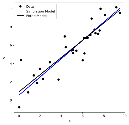
簡単にフィッティングする
ここで,(x,y)個のデータ点を1本の線でフィッティングする.(x,y)データ点をシミュレーションし,一定の不確実性を持つ真の例を示す.
import numpy as np
import matplotlib.pyplot as plt
from astropy.modeling import models, fitting

# define a model for a line
line_orig = models.Linear1D(slope=1.0, intercept=0.5)

# generate x, y data non-uniformly spaced in x
# add noise to y measurements
npts = 30
np.random.seed(10)
x = np.random.uniform(0.0, 10.0, npts)
y = line_orig(x)
yunc = np.absolute(np.random.normal(0.5, 2.5, npts))
y += np.random.normal(0.0, yunc, npts)

# initialize a linear fitter
fit = fitting.LinearLSQFitter()

# initialize a linear model
line_init = models.Linear1D()

# fit the data with the fitter
fitted_line = fit(line_init, x, y)

# plot
plt.figure()
plt.plot(x, y, 'ko', label='Data')
plt.plot(x, line_orig(x), 'b-', label='Simulation Model')
plt.plot(x, fitted_line(x), 'k-', label='Fitted Model')
plt.xlabel('x')
plt.ylabel('y')
plt.legend()

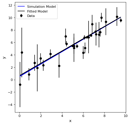
不確実性を使ってフィッティングする
重みとして不確定度を用いてフィッティングすることができる.ガウス誤差の場合の標準重み1/UNC^2を得るために、部品に渡す重みは1/UNCである。
import numpy as np
import matplotlib.pyplot as plt
from astropy.modeling import models, fitting

# define a model for a line
line_orig = models.Linear1D(slope=1.0, intercept=0.5)

# generate x, y data non-uniformly spaced in x
# add noise to y measurements
npts = 30
np.random.seed(10)
x = np.random.uniform(0.0, 10.0, npts)
y = line_orig(x)
yunc = np.absolute(np.random.normal(0.5, 2.5, npts))
y += np.random.normal(0.0, yunc, npts)

# initialize a linear fitter
fit = fitting.LinearLSQFitter()

# initialize a linear model
line_init = models.Linear1D()

# fit the data with the fitter
fitted_line = fit(line_init, x, y, weights=1.0/yunc)

# plot
plt.figure()
plt.errorbar(x, y, yerr=yunc, fmt='ko', label='Data')
plt.plot(x, line_orig(x), 'b-', label='Simulation Model')
plt.plot(x, fitted_line(x), 'k-', label='Fitted Model')
plt.xlabel('x')
plt.ylabel('y')
plt.legend()

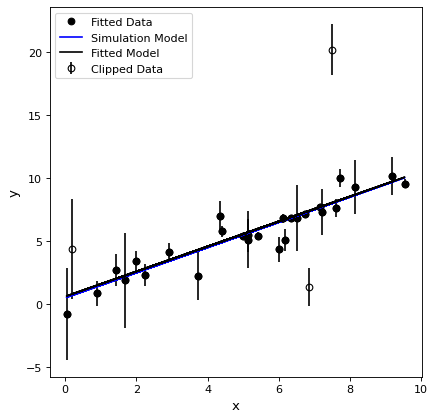
Sigma裁断を用いた反復フィッティング
フィッティング時には,フィッティングからの群外値データが存在する可能性があり,これらのデータはフィッティングに有意なばらつきを生じる可能性がある。これらのオフライン値は、識別され、適合から反復的に除去されることができる。反復σトリミングは、すべてのデータがσトリミング決定に対して同じ不確実性を有すると仮定することに留意されたい。
import numpy as np
import matplotlib.pyplot as plt
from astropy.stats import sigma_clip
from astropy.modeling import models, fitting

# define a model for a line
line_orig = models.Linear1D(slope=1.0, intercept=0.5)

# generate x, y data non-uniformly spaced in x
# add noise to y measurements
npts = 30
np.random.seed(10)
x = np.random.uniform(0.0, 10.0, npts)
y = line_orig(x)
yunc = np.absolute(np.random.normal(0.5, 2.5, npts))
y += np.random.normal(0.0, yunc, npts)

# make true outliers
y[3] = line_orig(x[3]) + 6 * yunc[3]
y[10] = line_orig(x[10]) - 4 * yunc[10]

# initialize a linear fitter
fit = fitting.LinearLSQFitter()

# initialize the outlier removal fitter
or_fit = fitting.FittingWithOutlierRemoval(fit, sigma_clip, niter=3, sigma=3.0)

# initialize a linear model
line_init = models.Linear1D()

# fit the data with the fitter
fitted_line, mask = or_fit(line_init, x, y, weights=1.0/yunc)
filtered_data = np.ma.masked_array(y, mask=mask)

# plot
plt.figure()
plt.errorbar(x, y, yerr=yunc, fmt="ko", fillstyle="none", label="Clipped Data")
plt.plot(x, filtered_data, "ko", label="Fitted Data")
plt.plot(x, line_orig(x), 'b-', label='Simulation Model')
plt.plot(x, fitted_line(x), 'k-', label='Fitted Model')
plt.xlabel('x')
plt.ylabel('y')
plt.legend()