モデルをデータにフィッティングします
このモジュールはFittersと呼ばれるNumpyとScipy適合関数のラッパを提供する。すべてのFitterは関数として呼び出すことができる.彼らは一例を挙げました FittableModel 入力として修正します parameters 属性です。このような考え方はスケーラビリティを持たせ,ユーザが他の治具を容易に追加できるようにすることである.
Numpy‘sを用いて線形フィッティングを行う numpy.linalg.lstsq 機能します。現在2つの非線形組み立て工が使用しています scipy.optimize.leastsq そして scipy.optimize.fmin_slsqp それがそうです。
入力をクランプに渡すルールには、
非線形チューブは現在単一のモデルにしか適用されていない(モデルセットには適用されない)。
線形フィッティングは、単一の入力を、複数の適合モデルを作成する複数のモデルセットに適合させることができる。これには指定が必要かもしれません
model_set_axisパラメータは,モデルを評価する際に使用するように;これは入力データをどのようにブロードキャストするかを知る必要があるかもしれない.♪the
LinearLSQFitter現在は単純(複合ではない)モデルにのみ適用されている.現在のフィッティング者は単一の出力を持つモデル(例えば二元関数を含む)のみを使用しています
Chebyshev2Dしかしマッピングの複合モデルではありませんx, y -> x', y')。
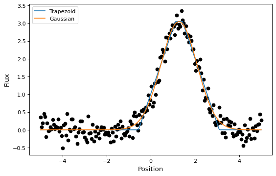
簡単な一次元モデルフィッティング
本節では、ガウス関数をアナログデータセットに適合させる簡単な例を示す。私たちが使うのは Gaussian1D そして Trapezoid1D モデルと LevMarLSQFitter データに適しています
import numpy as np
import matplotlib.pyplot as plt
from astropy.modeling import models, fitting

# Generate fake data
np.random.seed(0)
x = np.linspace(-5., 5., 200)
y = 3 * np.exp(-0.5 * (x - 1.3)**2 / 0.8**2)
y += np.random.normal(0., 0.2, x.shape)

# Fit the data using a box model.
# Bounds are not really needed but included here to demonstrate usage.
t_init = models.Trapezoid1D(amplitude=1., x_0=0., width=1., slope=0.5,
                            bounds={"x_0": (-5., 5.)})
fit_t = fitting.LevMarLSQFitter()
t = fit_t(t_init, x, y)

# Fit the data using a Gaussian
g_init = models.Gaussian1D(amplitude=1., mean=0, stddev=1.)
fit_g = fitting.LevMarLSQFitter()
g = fit_g(g_init, x, y)

# Plot the data with the best-fit model
plt.figure(figsize=(8,5))
plt.plot(x, y, 'ko')
plt.plot(x, t(x), label='Trapezoid')
plt.plot(x, g(x), label='Gaussian')
plt.xlabel('Position')
plt.ylabel('Flux')
plt.legend(loc=2)
以上のように,インスタンス化すると,Fitterクラスは初期モデルを受け取る関数として用いることができる. (t_init あるいは…。 g_init )とデータ値 (x そして y )を適合させたモデルに戻ります (t あるいは…。 g )。
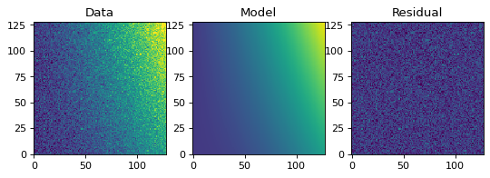
簡単な2次元モデルフィッティング
1−D例と同様に、シミュレーションされた2−Dデータセットを作成し、多項式モデルをデータセットに適合させることができる。例えば、これは、画像中の背景に適応するために使用されてもよい。
import warnings
import numpy as np
import matplotlib.pyplot as plt
from astropy.modeling import models, fitting

# Generate fake data
np.random.seed(0)
y, x = np.mgrid[:128, :128]
z = 2. * x ** 2 - 0.5 * x ** 2 + 1.5 * x * y - 1.
z += np.random.normal(0., 0.1, z.shape) * 50000.

# Fit the data using astropy.modeling
p_init = models.Polynomial2D(degree=2)
fit_p = fitting.LevMarLSQFitter()

with warnings.catch_warnings():
    # Ignore model linearity warning from the fitter
    warnings.simplefilter('ignore')
    p = fit_p(p_init, x, y, z)

# Plot the data with the best-fit model
plt.figure(figsize=(8, 2.5))
plt.subplot(1, 3, 1)
plt.imshow(z, origin='lower', interpolation='nearest', vmin=-1e4, vmax=5e4)
plt.title("Data")
plt.subplot(1, 3, 2)
plt.imshow(p(x, y), origin='lower', interpolation='nearest', vmin=-1e4,
           vmax=5e4)
plt.title("Model")
plt.subplot(1, 3, 3)
plt.imshow(z - p(x, y), origin='lower', interpolation='nearest', vmin=-1e4,
           vmax=5e4)
plt.title("Residual")
