マークと芸術家を重ね合わせて
次のページの例については、ここから紹介した例から始めましょう 世界座標初期化軸を用いて それがそうです。
画素座標.
Apart from the handling of the ticks, tick labels, and grid lines, the
WCSAxes class behaves like a normal Matplotlib
Axes instance, and methods such as
imshow(),
contour(),
plot(),
scatter(), and so on will work and plot the
data in pixel coordinates by default.
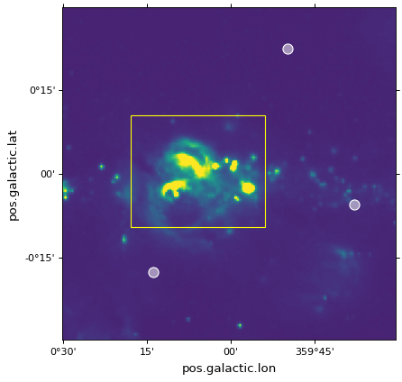
以下の例では、散布マークおよび矩形は、画素座標でプロットされる。
# The following line makes it so that the zoom level no longer changes,
# otherwise Matplotlib has a tendency to zoom out when adding overlays.
ax.set_autoscale_on(False)

# Add a rectangle with bottom left corner at pixel position (30, 50) with a
# width and height of 60 and 50 pixels respectively.
from matplotlib.patches import Rectangle
r = Rectangle((30., 50.), 60., 50., edgecolor='yellow', facecolor='none')
ax.add_patch(r)

# Add three markers at (40, 30), (100, 130), and (130, 60). The facecolor is
# a transparent white (0.5 is the alpha value).
ax.scatter([40, 100, 130], [30, 130, 60], s=100, edgecolor='white', facecolor=(1, 1, 1, 0.5))
世界座標.
このようなMatplotlibコマンドはすべて許可されています transform= パラメータは、入力をMatplotlibに渡し、描画する前に、入力をworldから画素座標に変換する。例えば:
ax.scatter(..., transform=...)
採用を伝えることができます scatter() 使用を伝えることができます transform= 最終的な画素座標を得る。
♪the WCSAxes クラスは1つを含む get_transform() 方法では、様々な世界座標系からMatplotlibに変換するために必要な最終画素座標系に変換するために、適切な変換オブジェクトを取得するために使用することができる。♪the get_transform() 方法は、複数の異なる入力を受け入れることができ、これを本部分および後続部分で紹介する。この方法の最も簡単な2つの入力は 'world' そして 'pixel' それがそうです。
例えば、WCSが角度(度単位)と波長(ナノ単位)とからなる座標系が画像を定義している場合、以下の動作を実行することができる。
ax.scatter([34], [3.2], transform=ax.get_transform('world'))
(34°,3.2 nm)に標識をプロットした。
Vbl.使用 ax.get_transform('pixel') 何の変換も使わないことに相当します Pixel coordinates 第(1)項。
天球座標
WCSが天球座標を表す特殊な場合には,他の多くの入力を渡すことができる. get_transform() それがそうです。これらは
'fk4':b 1950 FK 4赤道座標'fk5':J 2000 FK 5赤道座標'icrs':ICRS赤道座標'galactic':銀河座標
さらに効果的なものは astropy.coordinates 座標フレームを伝達することができる.
例えば、以下のコマンドを使用して、FK 5システムで定義された位置を有するフラグを追加することができます。
ax.scatter(266.78238, -28.769255, transform=ax.get_transform('fk5'), s=300,
           edgecolor='white', facecolor='none')
.の場合 scatter() そして plot() マークの中心位置は変換されるが,マーカ自体は画像の参照フレームに描画されており,これは歪んでいないように見えることを意味する.
パッチ/形状/ライン
変換はAstropyやMatplotlibパッチにも渡すことができる.例えば私たちは get_transform() 上の方法はFK 5赤道座標で四角形を描きます
from astropy import units as u
from astropy.visualization.wcsaxes import Quadrangle

r = Quadrangle((266.0, -28.9)*u.deg, 0.3*u.deg, 0.15*u.deg,
               edgecolor='green', facecolor='none',
               transform=ax.get_transform('fk5'))
ax.add_patch(r)
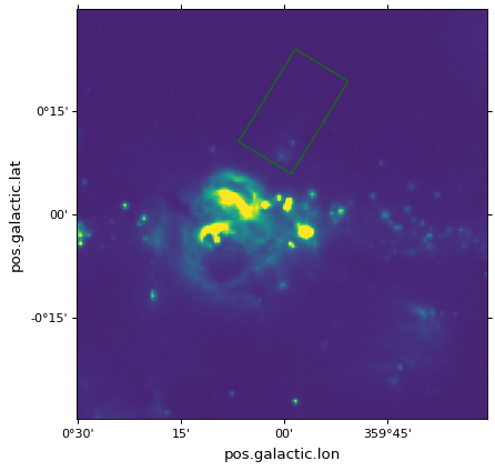
この場合、四角形は、FK 5 J 2000座標(266°,−28.9°)に印刷される。ご参照ください Quadrangles 部分的には,以下の内容に関するより多くの情報を知る. Quadrangle それがそうです。
しかしそれは 非常に重要です 高さは確かに0.15度となるが、幅は空の0.3度を厳密に表すのではなく、経度0.3度の間隔であることに注意されたい(緯度によっては空の異なる角度を表す)。すなわち、幅と高さが同じ値に設定されている場合には、生成されるポリゴンは正方形ではない。これは同様に Circle Patchこれは円を作ることはありません
from matplotlib.patches import Circle

r = Quadrangle((266.4, -28.9)*u.deg, 0.3*u.deg, 0.3*u.deg,
               edgecolor='cyan', facecolor='none',
               transform=ax.get_transform('fk5'))
ax.add_patch(r)

c = Circle((266.4, -29.1), 0.15, edgecolor='yellow', facecolor='none',
           transform=ax.get_transform('fk5'))
ax.add_patch(c)
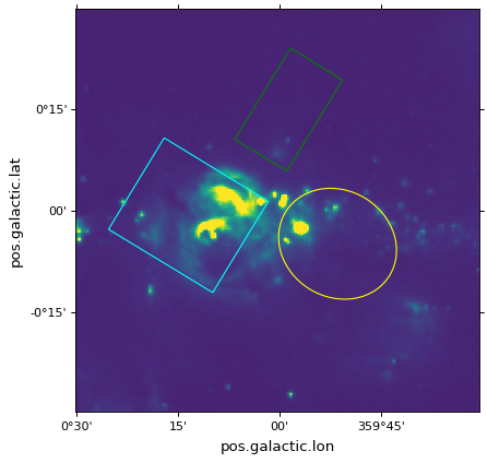
重要
ソースの周りに丸を描いて強調表示するだけで興味があれば、使用をお勧めします scatter() なぜなら、円形マーク(デフォルト設定)については、円は描画中の円として保証され、中心の位置のみが変換されるからである。
“真”球面円を描くには、ご覧ください Spherical patches 一節です。
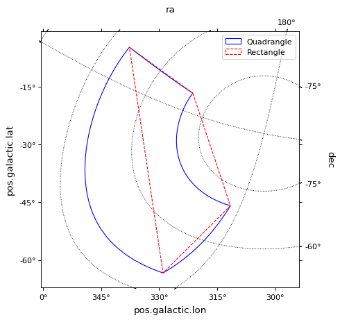
四合院
Quadrangle Matplotlibのパッチではなく、四角形を描く推奨パッチです。 Rectangle それがそうです。四角形の辺は、2つの一定経度の直線および2つの定緯度の直線上に位置する(または、関心のある座標系における等価部材名、例えば、右緯度および赤緯)。の縁 Quadrangle WCS変換に適用すると曲線にレンダリングされる.対照的に Rectangle いつもまっすぐな縁があります。以下に四角形を描く2種類のパッチタイプの比較を示す. ICRS 座標が開く Galactic 軸:
from matplotlib.patches import Rectangle

# Set the Galactic axes such that the plot includes the ICRS south pole
ax = plt.subplot(projection=wcs)
ax.set_xlim(0, 10000)
ax.set_ylim(-10000, 0)

# Overlay the ICRS coordinate grid
overlay = ax.get_coords_overlay('icrs')
overlay.grid(color='black', ls='dotted')

# Add a quadrangle patch (100 degrees by 20 degrees)
q = Quadrangle((255, -70)*u.deg, 100*u.deg, 20*u.deg,
               label='Quadrangle', edgecolor='blue', facecolor='none',
               transform=ax.get_transform('icrs'))
ax.add_patch(q)

# Add a rectangle patch (100 degrees by 20 degrees)
r = Rectangle((255, -70), 100, 20,
              label='Rectangle', edgecolor='red', facecolor='none', linestyle='--',
              transform=ax.get_transform('icrs'))
ax.add_patch(r)

plt.legend(loc='upper right')

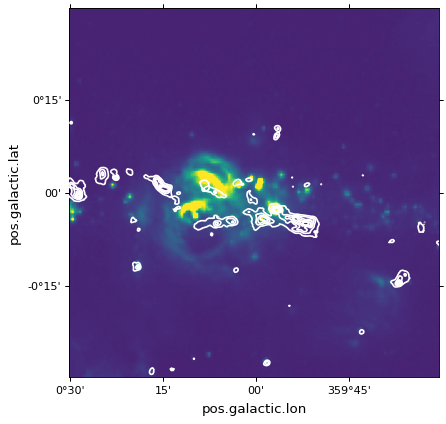
等高線.
等高線を重ね合わせるのも簡単です get_transform() 方法です。等高線に対しては get_transform() 画像のWCSは、その等高線を描画するために提供されるべきである。
filename = get_pkg_data_filename('galactic_center/gc_bolocam_gps.fits')
hdu = fits.open(filename)[0]
ax.contour(hdu.data, transform=ax.get_transform(WCS(hdu.header)),
           levels=[1,2,3,4,5,6], colors='white')
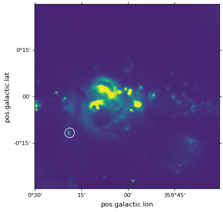
球面パッチ.
天文画像の描画中であり、ある経度/緯度の特定の角度内の面積を表す円を描きたい場合、 Circle 面片は歪んだ形状をもたらすため不適切である(経度と空の角度が異なるため)。この用例については、変更することができます SphericalCircle タプルが必要です Quantity 入力として、そして1つは Quantity 半径として:
from astropy import units as u
from astropy.visualization.wcsaxes import SphericalCircle

r = SphericalCircle((266.4 * u.deg, -29.1 * u.deg), 0.15 * u.degree,
                     edgecolor='yellow', facecolor='none',
                     transform=ax.get_transform('fk5'))
ax.add_patch(r)
