物理モデル.¶

これらのモデルは物理的に駆動されており，通常は物理問題の解決策として用いられている.これは，数学的動機から，通常数学問題の解決策である数学的動機とは対照的である.

BlackBody¶

♪the BlackBody モデルを使用するために Planck's Law それがそうです。黒体関数は

\[B_{\nu}(T)=A\frac{2 h\nu^{3}/c^{2}{exp(h\nu/k T)-1}\]

どこだ？ \(\nu\) 周波数です \(T\) 温度です \(A\) スケールファクタです \(h\) プラック定数です \(c\) 光速ですそして \(k\) ボルツマン定数です。

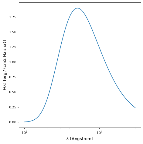
モデルの2つのパラメータはスケーリング係数である scale (A)と絶対温度 temperature (T).もし…。 scale 因子単位がなければ，結果はスペクトル放射単位，特にergs/(cm^2 Hz s Sr)であった。もし…。 scale 因子がスペクトル放射単位と共に伝達されると、結果はこれらの単位(例えば、ergs/(cm^2 A s Sr)またはmJy/Sr)で表される。設ける scale 単位がergs/(cm^2 A s Sr)である因子はプランク関数を与える. \(B_\lambda\) それがそうです。温度は任意の支持された温度単位で量として伝達することができる。

以下に温度10000 K，目盛り1の黒体の一例を示す.目盛りが1であることは，Planck関数が返されたデフォルト単位を用いてスケーリングされていないことを表す. BlackBody それがそうです。

import numpy as np
import matplotlib.pyplot as plt

from astropy.modeling.models import BlackBody
import astropy.units as u

wavelengths = np.logspace(np.log10(1000), np.log10(3e4), num=1000) * u.AA

# blackbody parameters
temperature = 10000 * u.K

# BlackBody provides the results in ergs/(cm^2 Hz s sr) when scale has no units
bb = BlackBody(temperature=temperature, scale=10000.0)
bb_result = bb(wavelengths)

fig, ax = plt.subplots(ncols=1)
ax.plot(wavelengths, bb_result, '-')

ax.set_xscale('log')
ax.set_xlabel(fr"$\lambda$ [{wavelengths.unit}]")
ax.set_ylabel(fr"$F(\lambda)$ [{bb_result.unit}]")

plt.tight_layout()
plt.show()

(png, svg, pdf)

♪the bolometric_flux() メンバーシップ関数は以下の式を用いて放射熱流束を測定する。 \(\sigma T^4/\pi\) どこだ？ \(\sigma\) ステファン·ボルツマン定数です

♪the lambda_max() そして nu_max() メンバーシップ関数が与える最大波長と周波数は \(B_\lambda\) そして \(B_\nu\) 別々に使います Wien's Law それがそうです。

旧黒体モジュールの注記について¶

V 4.0の前に黒体機能は astropy.modeling.blackbody モジュールは、その後、V 4.3で削除される。削除されたものをまだ使用している場合 blackbody モジュール、参照 Blackbody Module (deprecated capabilities) それがそうです。

ドルード1 D¶

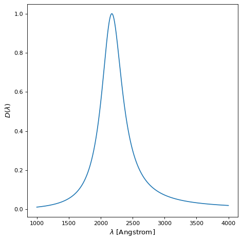
♪the Drude1D モデルは材料中の電子挙動のモデルを提供する(参照 Drude Model )である。まるで Lorentz1D モデルドルダーモデルはより広い翼比を持っています Gaussian1D モデルです。ドルダー断面は、2175オングストローム消光特性および中赤外芳香/多環芳香族炭化水素特徴を含む塵埃特徴をシミュレートするために使用されている。Drude関数です \(x\) はい。

\[D(X)=A\frac{(f/x_0)^2}{((x/x_0-x_0/x)^2+(f/x_0)^2}\]

どこだ？ \(A\) 振幅です \(f\) 最大値の半分の全幅で \(x_0\) 中心波長です。以下の機能を有するDrude 1 Dモデルの一例 \(x_0 = 2175\) アグストロムと \(f = 400\) Angstromを次の図に示す.

import numpy as np
import matplotlib.pyplot as plt

from astropy.modeling.models import Drude1D
import astropy.units as u

wavelengths = np.linspace(1000, 4000, num=1000) * u.AA

# Parameters and model
mod = Drude1D(amplitude=1.0, x_0=2175. * u.AA, fwhm=400. * u.AA)
mod_result = mod(wavelengths)

fig, ax = plt.subplots(ncols=1)
ax.plot(wavelengths, mod_result, '-')

ax.set_xlabel(fr"$\lambda$ [{wavelengths.unit}]")
ax.set_ylabel(r"$D(\lambda)$")

plt.tight_layout()
plt.show()

(png, svg, pdf)

NFW¶

♪the NFW モデルは1次元Navarro-Frenk-Whiteプロファイルを計算する.NFW断面における暗黒物質密度は以下の式で与えられる。

\[\rho(R)=\frac{\Delta_c\rho_{c}{r/r_s(1+r/r_s)^2}\]

どこだ？ \(\rho_{{c}}\) 輪郭が赤くずれたときの宇宙の臨界密度です \(\delta_c\) 超密度で \(r_s\) 輪郭の比例半径です。

このモデルは3つのパラメータに依存する：

mass ：輪郭の質量(単位が提供されていない場合は太陽質量で表す)

concentration ：プロファイルセット

redshift ：輪郭の赤移動

2つのオプションの初期化変数：

massfactor ：過密度タイプおよび因子を指定するタプルまたは文字列(デフォルト値(“Critical”、200))

cosmo ：密度計算の宇宙学(DEFAULT_COSMISTYとデフォルト)

注釈

評価前にNFWプロファイルオブジェクト(質量超密度と宇宙学を設定するため)を初期化する必要がある。

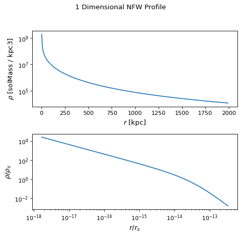
以下のパラメータを持つNFWプロファイルの様子を以下に示す.

mass = \(2.0 x 10^{15} M_{sun}\)

concentration =8.5

redshift =0.63

第1のグラフは半径としてNFW断面密度の関数である。第2の印刷は、NFW比例密度および比例半径で規格化された輪郭密度および半径をそれぞれ示す。スケール密度とスケール半径を属性として提供する rho_s そして r_s 超密度半径は通過可能です r_virial それがそうです。

import numpy as np
import matplotlib.pyplot as plt
from astropy.modeling.models import NFW
import astropy.units as u
from astropy import cosmology

# NFW Parameters
mass = u.Quantity(2.0E15, u.M_sun)
concentration = 8.5
redshift = 0.63
cosmo = cosmology.Planck15
massfactor = ("critical", 200)

# Create NFW Object
n = NFW(mass=mass, concentration=concentration, redshift=redshift, cosmo=cosmo,
        massfactor=massfactor)

# Radial distribution for plotting
radii = range(1,2001,10) * u.kpc

# Radial NFW density distribution
n_result = n(radii)

# Plot creation
fig, ax = plt.subplots(2)
fig.suptitle('1 Dimensional NFW Profile')

# Density profile subplot
ax[0].plot(radii, n_result, '-')
ax[0].set_yscale('log')
ax[0].set_xlabel(fr"$r$ [{radii.unit}]")
ax[0].set_ylabel(fr"$\rho$ [{n_result.unit}]")

# Create scaled density / scaled radius subplot
# NFW Object
n = NFW(mass=mass, concentration=concentration, redshift=redshift, cosmo=cosmo,
        massfactor=massfactor)

# Radial distribution for plotting
radii = np.logspace(np.log10(1e-5), np.log10(2), num=1000) * u.Mpc
n_result = n(radii)

# Scaled density / scaled radius subplot
ax[1].plot(radii / n.radius_s, n_result / n.density_s, '-')
ax[1].set_xscale('log')
ax[1].set_yscale('log')
ax[1].set_xlabel(r"$r / r_s$")
ax[1].set_ylabel(r"$\rho / \rho_s$")

# Display plot
plt.tight_layout(rect=[0, 0.03, 1, 0.95])
plt.show()

(png, svg, pdf)

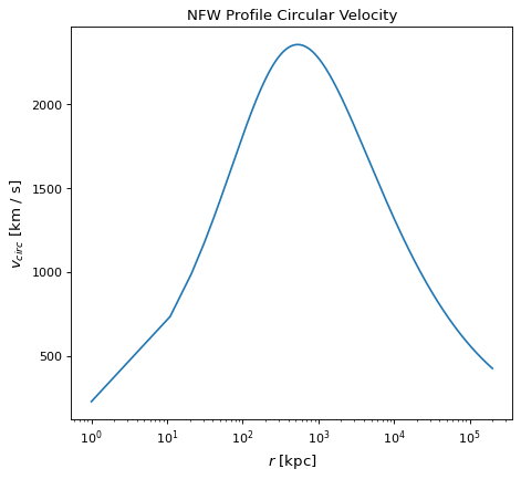
♪the circular_velocity() メンバーは位置ごとの円周速度を提供します r 方程式を使って

\[V_{cic}(R)^2=\frac{1}{x}\frac{\ln(1+cx)-(Cx)/(1+cx)}{\ln(1+c)-c/(1+c)}\]

where x is the ratio r\(/r_{vir}\). Circular velocities are provided in km/s.

以下のパラメータを有するNFW輪郭の円周速度例を以下に示す。

mass = \(2.0 x 10^{15} M_{sun}\)

concentration =8.5

redshift =0.63

属性としては，最大円周速度と最大周速度半径を用いることができる. v_max そして r_max それがそうです。

import matplotlib.pyplot as plt
from astropy.modeling.models import NFW
import astropy.units as u
from astropy import cosmology

# NFW Parameters
mass = u.Quantity(2.0E15, u.M_sun)
concentration = 8.5
redshift = 0.63
cosmo = cosmology.Planck15
massfactor = ("critical", 200)

# Create NFW Object
n = NFW(mass=mass, concentration=concentration, redshift=redshift, cosmo=cosmo,
        massfactor=massfactor)

# Radial distribution for plotting
radii = range(1,200001,10) * u.kpc

# NFW circular velocity distribution
n_result = n.circular_velocity(radii)

# Plot creation
fig,ax = plt.subplots()
ax.set_title('NFW Profile Circular Velocity')
ax.plot(radii, n_result, '-')
ax.set_xscale('log')
ax.set_xlabel(fr"$r$ [{radii.unit}]")
ax.set_ylabel(r"$v_{circ}$" + f" [{n_result.unit}]")

# Display plot
plt.tight_layout(rect=[0, 0.03, 1, 0.95])
plt.show()

(png, svg, pdf)

ナビゲーション

物理モデル.¶

BlackBody¶

旧黒体モジュールの注記について¶

ドルード1 D¶

NFW¶