時系列. (astropy.timeseries ）

序言：序言

固定時間サンプリング連続変数から計算時間窓内のイベントまで，天体物理学の多くの異なる領域で1次元時系列データを扱う必要がある.このニーズを満たすためには astropy.timeseries サブパケットは、時系列および動作時系列を表すクラスを提供する。

次に与える時系列クラスは QTable 時間を表す特殊な列を持つサブクラス使用 Time 級友たち。ここで説明されている多くの機能は データテーブル. (astropy.table ） ここに適用される。しかし新しいクラスの主な目的は時系列に特化した機能を提供することである. QTable それがそうです。

スタート

本節では，時系列の読み取り，データへのアクセス，およびいくつかの基本分析の実行を高速に理解する.時系列の作成と使用についての詳細は、参照 Vbl.使用 timeseries それがそうです。

最も基本的な時系列クラスは TimeSeries −時系列を特定の時点の値のセットとして表す。時系列を離散時間ボックス内のメトリックとして表現することに興味があれば、あなたはそうかもしれません BinnedTimeSeries 私たちが示しているサブクラスは Vbl.使用 timeseries ）。

まずケプラー光源曲線を含むFITSファイルを検索します

>>> from astropy.utils.data import get_pkg_data_filename
>>> filename = get_pkg_data_filename('timeseries/kplr010666592-2009131110544_slc.fits')  

注釈

ここで提供される照明曲線は、例示的な目的のために手動で選択される。ケプラー配合フォーマットの詳細については、ご参照ください Kepler Data Validation Document ケプラー科学センターと Light Curve Files 書類です。Pythonを使用して科学目的のための他のケプラー光線曲線を取得するには、参照されたい astroquery 付属小包です。

そして私たちは TimeSeries このファイルで読み込むクラス：

>>> from astropy.timeseries import TimeSeries
>>> ts = TimeSeries.read(filename, format='kepler.fits')  

時系列は特別な時系列である Table 対象：：

>>> ts  
<TimeSeries length=14280>
          time             timecorr   ...   pos_corr1      pos_corr2
                              d       ...      pix            pix
         object            float32    ...    float32        float32
----------------------- ------------- ... -------------- --------------
2009-05-02T00:41:40.338  6.630610e-04 ...  1.5822421e-03 -1.4463664e-03
2009-05-02T00:42:39.188  6.630857e-04 ...  1.5743829e-03 -1.4540013e-03
2009-05-02T00:43:38.045  6.631103e-04 ...  1.5665225e-03 -1.4616371e-03
2009-05-02T00:44:36.894  6.631350e-04 ...  1.5586632e-03 -1.4692718e-03
2009-05-02T00:45:35.752  6.631597e-04 ...  1.5508028e-03 -1.4769078e-03
2009-05-02T00:46:34.601  6.631844e-04 ...  1.5429436e-03 -1.4845425e-03
2009-05-02T00:47:33.451  6.632091e-04 ...  1.5350844e-03 -1.4921773e-03
2009-05-02T00:48:32.291  6.632337e-04 ...  1.5272264e-03 -1.4998110e-03
2009-05-02T00:49:31.149  6.632584e-04 ...  1.5193661e-03 -1.5074468e-03
                    ...           ... ...            ...            ...
2009-05-11T17:58:22.526  1.014493e-03 ...  3.6121816e-03  3.1950327e-03
2009-05-11T17:59:21.376  1.014518e-03 ...  3.6102540e-03  3.1872767e-03
2009-05-11T18:00:20.225  1.014542e-03 ...  3.6083264e-03  3.1795206e-03
2009-05-11T18:01:19.065  1.014567e-03 ...  3.6063993e-03  3.1717657e-03
2009-05-11T18:02:17.923  1.014591e-03 ...  3.6044715e-03  3.1640085e-03
2009-05-11T18:03:16.772  1.014615e-03 ...  3.6025438e-03  3.1562524e-03
2009-05-11T18:04:15.630  1.014640e-03 ...  3.6006160e-03  3.1484952e-03
2009-05-11T18:05:14.479  1.014664e-03 ...  3.5986886e-03  3.1407392e-03
2009-05-11T18:06:13.328  1.014689e-03 ...  3.5967610e-03  3.1329831e-03
2009-05-11T18:07:12.186  1.014713e-03 ...  3.5948332e-03  3.1252259e-03

…と同じ方法で Table 対象の各列と行 TimeSeries インデックス表現を使用してアクセスおよびスライスオブジェクトを使用することができる：

>>> ts['sap_flux']  
<Quantity [1027045.06, 1027184.44, 1027076.25, ..., 1025451.56, 1025468.5 ,
           1025930.9 ] electron / s>

>>> ts['time', 'sap_flux']  
<TimeSeries length=14280>
          time             sap_flux
                         electron / s
         object            float32
----------------------- --------------
2009-05-02T00:41:40.338  1.0270451e+06
2009-05-02T00:42:39.188  1.0271844e+06
2009-05-02T00:43:38.045  1.0270762e+06
2009-05-02T00:44:36.894  1.0271414e+06
2009-05-02T00:45:35.752  1.0271569e+06
2009-05-02T00:46:34.601  1.0272296e+06
2009-05-02T00:47:33.451  1.0273199e+06
2009-05-02T00:48:32.291  1.0271497e+06
2009-05-02T00:49:31.149  1.0271755e+06
                    ...            ...
2009-05-11T17:58:22.526  1.0234769e+06
2009-05-11T17:59:21.376  1.0234574e+06
2009-05-11T18:00:20.225  1.0238128e+06
2009-05-11T18:01:19.065  1.0243234e+06
2009-05-11T18:02:17.923  1.0244257e+06
2009-05-11T18:03:16.772  1.0248654e+06
2009-05-11T18:04:15.630  1.0250156e+06
2009-05-11T18:05:14.479  1.0254516e+06
2009-05-11T18:06:13.328  1.0254685e+06
2009-05-11T18:07:12.186  1.0259309e+06

>>> ts[0:4]  
<TimeSeries length=4>
          time             timecorr   ...   pos_corr1      pos_corr2
                              d       ...      pix            pix
         object            float32    ...    float32        float32
----------------------- ------------- ... -------------- --------------
2009-05-02T00:41:40.338  6.630610e-04 ...  1.5822421e-03 -1.4463664e-03
2009-05-02T00:42:39.188  6.630857e-04 ...  1.5743829e-03 -1.4540013e-03
2009-05-02T00:43:38.045  6.631103e-04 ...  1.5665225e-03 -1.4616371e-03
2009-05-02T00:44:36.894  6.631350e-04 ...  1.5586632e-03 -1.4692718e-03

先の例に示すように TimeSeries 相手が一人いる time 列は，その列はつねに第1列である.ご利用いただけます .time 属性：：

>>> ts.time  
<Time object: scale='tdb' format='isot' value=['2009-05-02T00:41:40.338' '2009-05-02T00:42:39.188'
  '2009-05-02T00:43:38.045' ... '2009-05-11T18:05:14.479'
  '2009-05-11T18:06:13.328' '2009-05-11T18:07:12.186']>

最初の列は常に Time 対象(参照) Times and Dates )したがって、異なる時間スケールおよびフォーマットに変換する機能をサポートする：

>>> ts.time.mjd  
array([54953.0289391 , 54953.02962023, 54953.03030145, ...,
       54962.7536398 , 54962.75432093, 54962.75500215])

>>> ts.time.unix  
array([1.24122483e+09, 1.24122489e+09, 1.24122495e+09, ...,
       1.24206505e+09, 1.24206511e+09, 1.24206517e+09])

時間がどの時間尺度に定義されているかを調べることもできます

>>> ts.time.scale  
'tdb'

重心動的時間目盛りでございます(ご覧ください 時間と日付 (astropy.time ） もっと詳しい情報を知っています)。これまで見てきたことを使ってストーリーを作ることができます

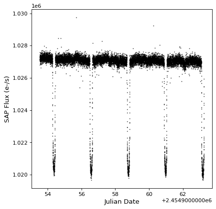
import matplotlib.pyplot as plt
plt.plot(ts.time.jd, ts['sap_flux'], 'k.', markersize=1)
plt.xlabel('Julian Date')
plt.ylabel('SAP Flux (e-/s)')

(png, svg, pdf)

いくつかの乗り換え駅があるようですね。私たちは使用することができます BoxLeastSquares クラスは、“ボックス最小二乗”(BLS)アルゴリズムを使用してサイクルを推定する：

>>> import numpy as np
>>> from astropy import units as u
>>> from astropy.timeseries import BoxLeastSquares
>>> periodogram = BoxLeastSquares.from_timeseries(ts, 'sap_flux')  

サイクルマップ解析を行うためには、持続時間0.2日の枠を使用します。

>>> results = periodogram.autopower(0.2 * u.day)  
>>> best = np.argmax(results.power)  
>>> period = results.period[best]  
>>> period  
<Quantity 2.20551724 d>
>>> transit_time = results.transit_time[best]  
>>> transit_time  
<Time object: scale='tdb' format='isot' value=2009-05-02T20:51:16.338>

利用可能な周期図アルゴリズムの詳細については，参照されたい 周期図アルゴリズム それがそうです。

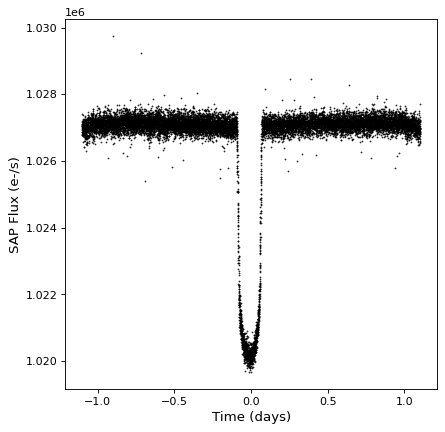
上で見つけた周期を使って時系列を折り畳むことができます fold() 方法：

>>> ts_folded = ts.fold(period=period, epoch_time=transit_time)  

折りたたんだ時系列を見てみましょう

plt.plot(ts_folded.time.jd, ts_folded['sap_flux'], 'k.', markersize=1)
plt.xlabel('Time (days)')
plt.ylabel('SAP Flux (e-/s)')

(png, svg, pdf)

使用 天体統計ツール (astropy.stats ） モジュールでは、ベースライン流量を決定するために、データをシグマトリミングすることによって流量を正規化することができる。

>>> from astropy.stats import sigma_clipped_stats
>>> mean, median, stddev = sigma_clipped_stats(ts_folded['sap_flux'])  
>>> ts_folded['sap_flux_norm'] = ts_folded['sap_flux'] / median  

点を等しい時間のボックスに入れることで、時系列をダウンサンプリングすることができます。これは1つに戻ります。 BinnedTimeSeries **

>>> from astropy.timeseries import aggregate_downsample
>>> ts_binned = aggregate_downsample(ts_folded, time_bin_size=0.03 * u.day)  
>>> ts_binned  
<BinnedTimeSeries length=74>
   time_bin_start     time_bin_size    ...   sap_flux_norm
                            s          ...
       object            float64       ...       float64
------------------- ------------------ ... ------------------
-1.1022116370482966             2592.0 ... 0.9998741745948792
-1.0722116370482966             2592.0 ... 0.9999074339866638
-1.0422116370482966             2592.0 ...  0.999972939491272
-1.0122116370482965             2592.0 ... 1.0000077486038208
-0.9822116370482965             2592.0 ... 0.9999921917915344
-0.9522116370482965             2592.0 ... 1.0000101327896118
-0.9222116370482966             2592.0 ... 1.0000121593475342
-0.8922116370482965             2592.0 ... 0.9999905228614807
-0.8622116370482965 2592.0000000000023 ... 1.0000263452529907
                ...                ... ...                ...
 0.8177883629517035 2591.9999999999977 ... 1.0000624656677246
 0.8477883629517035 2592.0000000000014 ... 1.0000633001327515
 0.8777883629517035  2592.000000000019 ... 1.0000433921813965
 0.9077883629517037 2591.9999999999814 ...  1.000024676322937
 0.9377883629517034   2592.00000000002 ... 1.0000224113464355
 0.9677883629517037  2591.999999999981 ... 1.0000698566436768
 0.9977883629517035             2592.0 ... 0.9999606013298035
 1.0277883629517035             2592.0 ... 0.9999635815620422
 1.0577883629517035             2592.0 ... 0.9999105930328369
 1.0877883629517036 2592.0000000000095 ... 0.9998687505722046

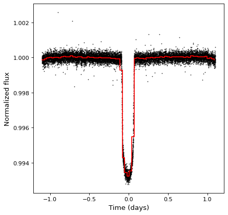
最終的な結果を見てみましょう

plt.plot(ts_folded.time.jd, ts_folded['sap_flux_norm'], 'k.', markersize=1)
plt.plot(ts_binned.time_bin_start.jd, ts_binned['sap_flux_norm'], 'r-', drawstyle='steps-post')
plt.xlabel('Time (days)')
plt.ylabel('Normalized flux')

(png, svg, pdf)

中の機能に関するより多くの情報を知るためには、以下の操作を実行してください astropy.timeseries モジュールでは，次節で完全文書へのリンクを見つけることができる.

Vbl.使用 timeseries

使用の詳細情報 astropy.timeseries 以下の各節で関連情報を提供する.

時系列の初期化と読み出し

• 時系列の作成
  • 時系列を初期化する
  • 入庫された時系列を初期化する
  • 時系列へのデータの追加
• 時系列を読み書きする
  • 内蔵カードリーダ
  • 通常の光線曲線形式を読む

アクセスデータと処理時系列

• 時系列のデータにアクセスする
  • データにアクセスする
  • 訪問時間.
  • 列子集を抽出する.
  • 行のサブセットを抽出する
• 異なる時間表現間で変換する
  • 時間を切り替える
  • 時間をフォーマットする.
  • 他の時間に対する時間
• 時系列の処理と解析
  • 時系列を組み合わせる
  • 時系列順序付け
  • 再サンプリングする.
  • 折り畳む
  • 算数をする.
• 時系列中のマスク値
  • 例を引く
• パンダセットとドッキングします
  • 例を引く

周期図アルゴリズム

• Lomb-Scarger周期図
  • 基本的用法
  • 周期図正規化
  • ピーク有意性と虚警告確率
  • 周期図アルゴリズム
  • RR天琴座例
  • 文献参考文献
• ボックス最小二乗(BLS)サイクルマップ
  • 数学的背景
  • 基本的用法
  • 目標.目標
  • 周期グリッド
  • ピーク統計情報
  • 文献参考文献

参照/API

Asterpy.TimeSeriesバッグ

このサブパケットは、時系列を処理するためのクラスおよび関数を含む。

機能

aggregate_downsample \(時間_シリーズ，*[, ...] )	時系列は、単一の関数を使用して固定サイズを有するボックスに値を結合することによって、ボックス内の値を結合することによってダウンサンプリングされる。
autocheck_required_columns \(CLS)	これは、テーブルが_REQUIRED_COLUMNS属性によって示される特定の方法を含むことを保証することができる装飾符である。

クラス

BasePeriodogram \(t，y[, dy] )
BaseTimeSeries \([data, masked, names, dtype, ...] )
BinnedTimeSeries \([data, time_bin_start, ...] )	バイナリ時系列データのクラスを表形式で表す.
BoxLeastSquares \(t，y[, dy] )	計算箱最小二乗周期図
BoxLeastSquaresResults \(*パラメータ)	BoxLeastSquare探索の結果
LombScargle \(t，y[, dy, fit_mean, ...] )	Lomb-Scarger周期図を計算する.
TimeSeries \([data, time, time_start, ...] )	時系列データのクラスを表形式で表す.

クラス継承関係図

Asterpy.timeseries.ioバッグ

機能

kepler_fits_reader \(ファイル名)

天体時系列におけるケプラーやコケファイルのFITSリーダとすることができる。