畳み込みとフィルタリング (astropy.convolution )
序言:序言
astropy.convolution 畳み込み関数とカーネルを提供し,SciPyに比べて改善を提供した. scipy.ndimage 畳み込みルーチンは、以下を含む。
NaN値を正しく処理する(畳み込みではこれらを無視し、NaN画素を補間値で置き換える)
1次元、2次元、3次元畳み込みの単一関数
エッジ処理オプションを改善しました
直接フーリエ変換(FFT)および高速フーリエ変換(FFT)バージョン
天文学でよく使われる内蔵カーネル
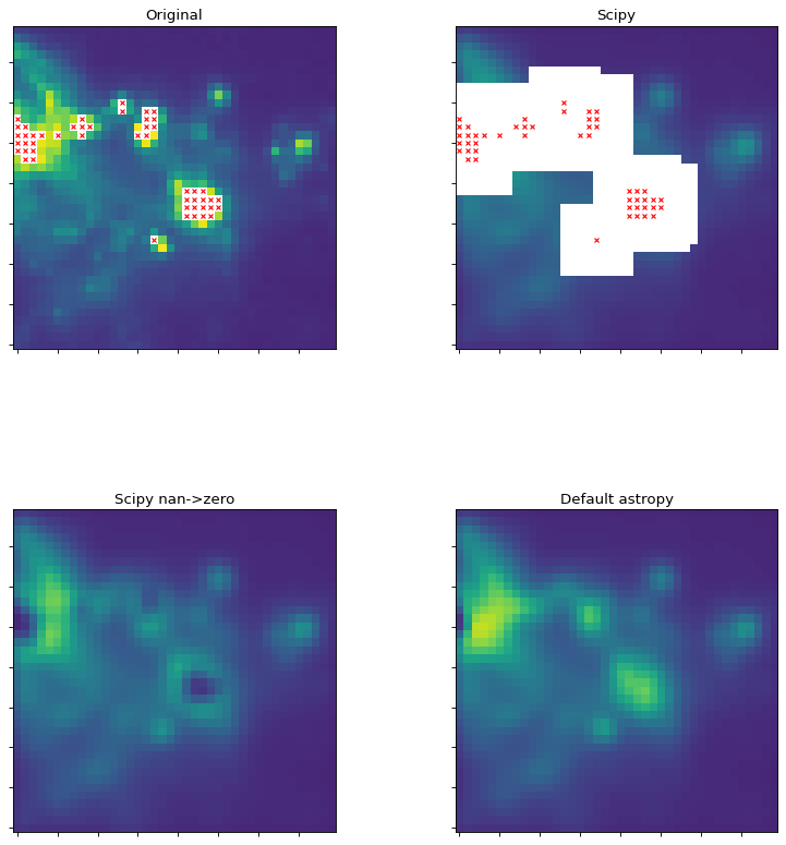
以下のサムネイルは scipy そして astropy NaN値を含む天文画像に対して畳み込み関数を行う. scipy 関数は、実質的に任意のNaN値のカーネル内のすべての画素に対してNaNを返すが、これは通常、予期される結果ではない。
import numpy as np
import matplotlib.pyplot as plt
from astropy.io import fits
from astropy.utils.data import get_pkg_data_filename
from astropy.convolution import Gaussian2DKernel
from scipy.signal import convolve as scipy_convolve
from astropy.convolution import convolve
# Load the data from data.astropy.org
filename = get_pkg_data_filename('galactic_center/gc_msx_e.fits')
hdu = fits.open(filename)[0]
# Scale the file to have reasonable numbers
# (this is mostly so that colorbars do not have too many digits)
# Also, we crop it so you can see individual pixels
img = hdu.data[50:90, 60:100] * 1e5
# This example is intended to demonstrate how astropy.convolve and
# scipy.convolve handle missing data, so we start by setting the
# brightest pixels to NaN to simulate a "saturated" data set
img[img > 2e1] = np.nan
# We also create a copy of the data and set those NaNs to zero. We will
# use this for the scipy convolution
img_zerod = img.copy()
img_zerod[np.isnan(img)] = 0
# We smooth with a Gaussian kernel with x_stddev=1 (and y_stddev=1)
# It is a 9x9 array
kernel = Gaussian2DKernel(x_stddev=1)
# Convolution: scipy's direct convolution mode spreads out NaNs (see
# panel 2 below)
scipy_conv = scipy_convolve(img, kernel, mode='same', method='direct')
# scipy's direct convolution mode run on the 'zero'd' image will not
# have NaNs, but will have some very low value zones where the NaNs were
# (see panel 3 below)
scipy_conv_zerod = scipy_convolve(img_zerod, kernel, mode='same',
method='direct')
# astropy's convolution replaces the NaN pixels with a kernel-weighted
# interpolation from their neighbors
astropy_conv = convolve(img, kernel)
# Now we do a bunch of plots. In the first two plots, the originally masked
# values are marked with red X's
plt.figure(1, figsize=(12, 12)).clf()
ax1 = plt.subplot(2, 2, 1)
im = ax1.imshow(img, vmin=-2., vmax=2.e1, origin='lower',
interpolation='nearest', cmap='viridis')
y, x = np.where(np.isnan(img))
ax1.set_autoscale_on(False)
ax1.plot(x, y, 'rx', markersize=4)
ax1.set_title("Original")
ax1.set_xticklabels([])
ax1.set_yticklabels([])
ax2 = plt.subplot(2, 2, 2)
im = ax2.imshow(scipy_conv, vmin=-2., vmax=2.e1, origin='lower',
interpolation='nearest', cmap='viridis')
ax2.set_autoscale_on(False)
ax2.plot(x, y, 'rx', markersize=4)
ax2.set_title("Scipy")
ax2.set_xticklabels([])
ax2.set_yticklabels([])
ax3 = plt.subplot(2, 2, 3)
im = ax3.imshow(scipy_conv_zerod, vmin=-2., vmax=2.e1, origin='lower',
interpolation='nearest', cmap='viridis')
ax3.set_title("Scipy nan->zero")
ax3.set_xticklabels([])
ax3.set_yticklabels([])
ax4 = plt.subplot(2, 2, 4)
im = ax4.imshow(astropy_conv, vmin=-2., vmax=2.e1, origin='lower',
interpolation='nearest', cmap='viridis')
ax4.set_title("Default astropy")
ax4.set_xticklabels([])
ax4.set_yticklabels([])
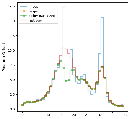
# we make a second plot of the amplitudes vs offset position to more
# clearly illustrate the value differences
plt.figure(2).clf()
plt.plot(img[:, 25], label='input', drawstyle='steps-mid', linewidth=2,
alpha=0.5)
plt.plot(scipy_conv[:, 25], label='scipy', drawstyle='steps-mid',
linewidth=2, alpha=0.5, marker='s')
plt.plot(scipy_conv_zerod[:, 25], label='scipy nan->zero',
drawstyle='steps-mid', linewidth=2, alpha=0.5, marker='s')
plt.plot(astropy_conv[:, 25], label='astropy', drawstyle='steps-mid',
linewidth=2, alpha=0.5)
plt.ylabel("Amplitude")
plt.ylabel("Position Offset")
plt.legend(loc='best')
plt.show()

以下の各節では,畳み込み関数をどのように用いるか,内蔵畳み込みカーネルをどのように用いるかについて述べる.
スタート
2つの畳み込み関数を提供した。これらは以下のように導入されています
from astropy.convolution import convolve, convolve_fft
そして両方として使われています
result = convolve(image, kernel)
result = convolve_fft(image, kernel)
convolve() 直接畳み込みアルゴリズムとして実現されています convolve_fft() 高速フーリエ変換(FFT)を用いる。したがって,前者は小さいカーネルに適用し,後者は大きなカーネルに適用した方がはるかに効率が良い.
例を引く
1次元データセットをユーザが指定したカーネルと畳み込みするためには,以下の操作を行うことができる.
>>> from astropy.convolution import convolve
>>> convolve([1, 4, 5, 6, 5, 7, 8], [0.2, 0.6, 0.2])
array([1.4, 3.6, 5. , 5.6, 5.6, 6.8, 6.2])
なお、端点がゼロに設定されているデフォルトの場合、境界に近すぎて畳み込み値を計算できない点はゼロに設定される。しかし、 convolve() 関数使用許可 boundary 代替行動のパラメータを指定するために使用することができる。例えば、設定 boundary='extend' 定数外挿法のみを用いて元のデータを境界外に拡張したと仮定すると,エッジ付近の値が計算される:
>>> from astropy.convolution import convolve
>>> convolve([1, 4, 5, 6, 5, 7, 8], [0.2, 0.6, 0.2], boundary='extend')
array([1.6, 3.6, 5. , 5.6, 5.6, 6.8, 7.8])
末尾の値は,1番目の点以下のいずれの値もであると仮定したものである. 1 最後の点よりも高い値は 8 それがそうです。境界処理に関するより詳細な議論は、参照されたい 畳み込み関数を用いる それがそうです。
例を引く
畳み込みモジュールは、例えば、以下のように導入することができる内蔵カーネルをさらに含む。
>>> from astropy.convolution import Gaussian1DKernel
カーネルを使用するためには、まず、カーネルの特定の例を作成してください:
>>> gauss = Gaussian1DKernel(stddev=2)
gauss 配列ではなく,カーネルオブジェクトである.利用可能::下位配列を検索する.
>>> gauss.array
array([6.69151129e-05, 4.36341348e-04, 2.21592421e-03,
       8.76415025e-03, 2.69954833e-02, 6.47587978e-02,
       1.20985362e-01, 1.76032663e-01, 1.99471140e-01,
       1.76032663e-01, 1.20985362e-01, 6.47587978e-02,
       2.69954833e-02, 8.76415025e-03, 2.21592421e-03,
       4.36341348e-04, 6.69151129e-05])
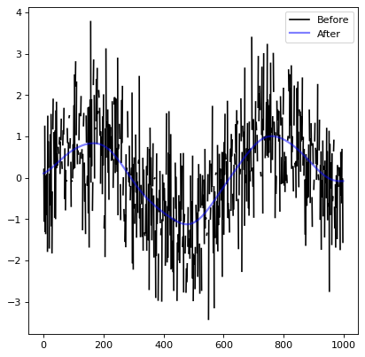
そして呼び出し時にカーネルを直接使用することができます convolve() :
import numpy as np
import matplotlib.pyplot as plt

from astropy.convolution import Gaussian1DKernel, convolve

plt.figure(3).clf()

# Generate fake data
x = np.arange(1000).astype(float)
y = np.sin(x / 100.) + np.random.normal(0., 1., x.shape)
y[::3] = np.nan

# Create kernel
g = Gaussian1DKernel(stddev=50)

# Convolve data
z = convolve(y, g)

# Plot data before and after convolution
plt.plot(x, y, 'k-', label='Before')
plt.plot(x, z, 'b-', label='After', alpha=0.5, linewidth=2)
plt.legend(loc='best')
plt.show()
Vbl.使用 astropy 悪いデータを置き換えるために畳み込みする
astropy この畳み込み方法は、隣接データから補間された値で悪いデータを置換することができ、コアベースの補間は、少量の不良画素を含む画像を処理することや、疎サンプリングされた画像を補間するために非常に有用である。
補間ツールの実現と利用方式は以下のとおりである.
from astropy.convolution import interpolate_replace_nans
result = interpolate_replace_nans(image, kernel)
カーネルベースの補間を使用することを望むことができるいくつかのコンテキストは、
画素が飽和した画像。一般に、これらの領域は撮像領域の中で最も強度の高い領域であり、補間は信頼できないが、これは表示に有用である。
マーキングされた画素を有する画像(例えば、宇宙線またはそれらの画素をマーキングする必要がある他の偽信号の影響を受けるいくつかの小領域)。影響された領域が十分に小さい場合、生成された補間は、ソース統計データに小さな影響を与え、得られたデータ上でロバストなソースルックアップアルゴリズムを実行することを可能にする可能性がある。
単一画素検出器を使用して構築された画像のような間引きサンプリング画像。このような画像は、撮像領域でいくつかの離散点のみがサンプリングされるが、拡張された空放射の近似値を構築することができる。
注釈
カーネルがNAN値の潜在的連続領域を完全にカバーするために十分に大きいことに注意しなければならない.一個 AstropyUserWarning 畳み込み後にNaN値が検出されると発火し,この場合にはカーネルサイズを増加させるべきである.
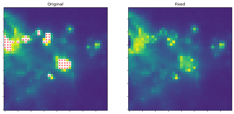
例を引く
以下のスクリプトは、マーキングされた画素を充填するためのカーネル補間例を示す。
import numpy as np
import matplotlib.pyplot as plt

from astropy.io import fits
from astropy.utils.data import get_pkg_data_filename
from astropy.convolution import Gaussian2DKernel, interpolate_replace_nans

# Load the data from data.astropy.org
filename = get_pkg_data_filename('galactic_center/gc_msx_e.fits')

hdu = fits.open(filename)[0]
img = hdu.data[50:90, 60:100] * 1e5

# This example is intended to demonstrate how astropy.convolve and
# scipy.convolve handle missing data, so we start by setting the brightest
# pixels to NaN to simulate a "saturated" data set
img[img > 2e1] = np.nan

# We smooth with a Gaussian kernel with x_stddev=1 (and y_stddev=1)
# It is a 9x9 array
kernel = Gaussian2DKernel(x_stddev=1)

# create a "fixed" image with NaNs replaced by interpolated values
fixed_image = interpolate_replace_nans(img, kernel)

# Now we do a bunch of plots.  In the first two plots, the originally masked
# values are marked with red X's
plt.figure(1, figsize=(12, 6)).clf()
plt.close(2) # close the second plot from above

ax1 = plt.subplot(1, 2, 1)
im = ax1.imshow(img, vmin=-2., vmax=2.e1, origin='lower',
                interpolation='nearest', cmap='viridis')
y, x = np.where(np.isnan(img))
ax1.set_autoscale_on(False)
ax1.plot(x, y, 'rx', markersize=4)
ax1.set_title("Original")
ax1.set_xticklabels([])
ax1.set_yticklabels([])

ax2 = plt.subplot(1, 2, 2)
im = ax2.imshow(fixed_image, vmin=-2., vmax=2.e1, origin='lower',
                interpolation='nearest', cmap='viridis')
ax2.set_title("Fixed")
ax2.set_xticklabels([])
ax2.set_yticklabels([])
例を引く
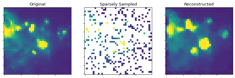
このスクリプトは,疎サンプリングから画像を再構成するためのこの技術の強力な機能を示している.画像は完璧ではありません:点状信号源は失われることがありますが、肉眼では拡張された構造をうまく回復することができます。
import numpy as np
import matplotlib.pyplot as plt

from astropy.io import fits
from astropy.utils.data import get_pkg_data_filename
from astropy.convolution import Gaussian2DKernel, interpolate_replace_nans

# Load the data from data.astropy.org
filename = get_pkg_data_filename('galactic_center/gc_msx_e.fits')

hdu = fits.open(filename)[0]
img = hdu.data[50:90, 60:100] * 1e5

indices = np.random.randint(low=0, high=img.size, size=300)

sampled_data = img.flat[indices]

# Build a new, sparsely sampled version of the original image
new_img = np.tile(np.nan, img.shape)
new_img.flat[indices] = sampled_data

# We smooth with a Gaussian kernel with x_stddev=1 (and y_stddev=1)
# It is a 9x9 array
kernel = Gaussian2DKernel(x_stddev=1)

# create a "reconstructed" image with NaNs replaced by interpolated values
reconstructed_image = interpolate_replace_nans(new_img, kernel)

# Now we do a bunch of plots.  In the first two plots, the originally masked
# values are marked with red X's
plt.figure(1, figsize=(12, 6)).clf()
ax1 = plt.subplot(1, 3, 1)
im = ax1.imshow(img, vmin=-2., vmax=2.e1, origin='lower',
                interpolation='nearest', cmap='viridis')
y, x = np.where(np.isnan(img))
ax1.set_autoscale_on(False)
ax1.set_title("Original")
ax1.set_xticklabels([])
ax1.set_yticklabels([])

ax2 = plt.subplot(1, 3, 2)
im = ax2.imshow(new_img, vmin=-2., vmax=2.e1, origin='lower',
                interpolation='nearest', cmap='viridis')
ax2.set_title("Sparsely Sampled")
ax2.set_xticklabels([])
ax2.set_yticklabels([])

ax2 = plt.subplot(1, 3, 3)
im = ax2.imshow(reconstructed_image, vmin=-2., vmax=2.e1, origin='lower',
                interpolation='nearest', cmap='viridis')
ax2.set_title("Reconstructed")
ax2.set_xticklabels([])
ax2.set_yticklabels([])

後方互換性(バージョン2.0以前のバージョン)についての説明
の行為です。 astropy の直接畳み込み (convolve() )は、バージョン2.0で変更されました。一般的に、古いバージョンは人気がありません。しかし高齢者の行動を回復するには (astropy 2.0版以下)直接畳み込み関数は、補間再畳み込み、例えば、:
from astropy.convolution import interpolate_replace_nans, convolve
interped_result = interpolate_replace_nans(image, kernel)
result = convolve(interped_image, kernel)
両者のデフォルト行動に注意してください convolve そして convolve_fft ショーです。 正規化畳み込み そして,その過程でNANを挿入する.この注釈で与えられた例と、以前に古いバージョンで直接畳み込みでのみ実行されていた動作 astropy 次に,NANを補間値で置き換え,すべての非NaN値を不変に保ちながら,指定されたカーネルで生成された画像を畳み込みする2ステップのプロセスを実行する.
Vbl.使用 astropy.convolution
性能提示
♪the convolve() 関数は小さいカーネルに最適であり,大きなカーネルに対して非常に遅くなる可能性がある.この場合,利用が考えられる convolve_fft() (ただし,この関数はより多くのメモリを使用していることに注意されたい).
参照/API
星座·畳み込みパッケージ
機能
|
配列とカーネルを畳み込みする. |
|
Ndarrayとn-カーネルを畳み込みする. |
|
畳み込み手法を用いて2つのモデルの畳み込みを行う |
|
畳み込み手法を用いて2つのモデルの畳み込みを行う |
|
メッシュ上の解析モデル関数を計算するための関数。 |
|
NANを含むデータセットが与えられ、NANは、所与のカーネルを有する隣接データ点から補間することによって置換される。 |
|
2つのカーネルを加算、減算、または乗算する。 |
クラス
|
2 D Aryディスクカーネル。 |
|
1次元ボックスフィルタカーネル。 |
|
2 D直方体フィルタコア。 |
|
フィルタカーネルは、リストまたは配列から作成されます。 |
|
一次元ガウスフィルタリングコア。 |
|
二次元ガウスフィルタリング核。 |
|
カーネルベースクラスを畳み込みする. |
|
1次元フィルタカーネルの基底クラス. |
|
2 Dフィルタコアの基本クラスです。 |
カーネルサイズが偶数の場合は呼び出される. |
|
|
1次元モデルからカーネルを作成する. |
|
2 Dモデルからカーネルを作成します。 |
|
2 D Moffatカーネル。 |
|
1 D Rickerウェーブレットフィルタリングコア(“メキシコキャップ”コアとも呼ばれることがあります)。 |
|
2 D Rickerウェーブレットフィルタリングカーネル(“メキシコキャップ”カーネルと呼ばれることもあります)。 |
|
2 Dリングフィルタコア。 |
|
2 D TOPHATフィルタコア。 |
|
一次元台形核。 |
|
二次元台形核。 |